|
Vanggaard, Morten Eghøj (s042365) |
Lund, Dan Toste (s031758) |
The input files for HOMER can be download at this link in
a zip file (0.7mb)
The full report in PDF can be download
at this link
(1.25mb)
This webpage is created in MS word and has some problemes with the
format. So the report in PDF has the
corrected layout.
The currency in this report is Danish
krones (kr. Or DKK). The exchange rate can be found at www.xe.com or Google.com .
Feel free to email comments.
Morten Eghøj 30.12.2009
Abstract
Background Off grid electrical power system has developed over the last years and the price of the systems has gone down. This makes it an option which is comparable with a grid connection. The off grid installation needs to be size correctly to a compatible option and this is done with a valid weather data source and refined demands curves.
Results The results has been computed with a simulation program and it has given results which has shown that the off grid system has different solutions, depending on the weather conditions in the cities where the system is installed and demand. It is shown that lowering the demand, gives a smaller system and is less depend of stable weather conditions.
Conclusion Off grid systems is an option in 3 cities in Greenland but it needs to be size correctly and the weather data makes it possible. Lowering the demand is a factory which should have focus, because it makes the system more attractive than grid connection.
Acknowledgements
Thanks to Bengt Perers (Danmarks Tekniske Universitet) which has been the supervisor on this project and has been available whenever needed and for making this project available.
Thanks to Jens Christian (certified
electrician) which has been kind to provide information about the grid in
Greenland and how the grid installation is made on Greenland.
Table of Content
Consumption with normal
appliances
Load/peak curve for
consumption with normal appliances.
Consumption with
efficient appliances and change of heat input
Load/peak curve with
efficient appliances and change of heat input
Simulation input from
services loads.
Off-grid system with a
household turbine
Simulations for Nuuk from
May to august month
Simulations for Sisimiut
from May to august month
Simulations for Uummannaq
from May to august month
Simulations for Nuuk,
from May to august month, with a household wind turbine
Simulations for Sismumt,
from May to august month, with a household wind turbine
Simulations for
Uummannaq, from May to august month, with a household wind turbine
Result for Breakeven grid distance
Appendix 4: System
Report - Nuuk_maj_august
1
Introduction
In this study the goal is to investigate the economics of building a “Standalone PV system” for Greenland and compare the results to a grid extension.
For this purpose some data are provided and
some information is assumed:
It is not stated who the user of the standalone PV system are therefore it is
assumed to be single family house with 2 adults and well equipped with technology
of different kind
Weather data from 3 places in Greenland: Nuuk, Sisimiut and Uummannaq. To help estimate cost and running economics a program, HOMER (Homer Energy), was used. It is not in detailed explained how to use the program, but all relevant information about input data are.
As one of the features in HOMER a small wind turbine was tried as a possibility for the system.
To visualize where in Greenland it is the cities are marked as, A: Nuuk, B: Sisimiut, C: Uummannaq and D: Copenhagen in fig 1.
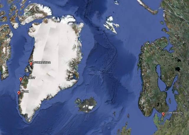
fig 1: Locations for PV stand alone systems and Copenhagen. - Screen print
from Google Earth
Off grid
A off grid system is designed to provide services that a home or business needs without electric supply from the grid. In this house the service is electricity supply and the power generation source is renewable energy. This is sources like sun, wind and bio fuel. The power source goes into the system and is output as electricity at the right condition.
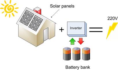
fig 2: Off grid system
The off grid system on fig 2 has three main parts. Solar panels, inverter and batteries. The solar panels generates direct current (DC) which is transform in the inverter into alternating current (AC) to be used in standard appliances. This is the outline for the system. On top of it a controller monitors the electrical input from the solar panels and controls charging of the battery bank. Depending on the system, the charge controller and inverter can be the same unit.
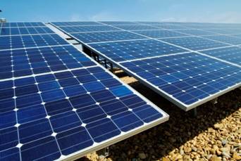
Solar panel
The solar panels are essential in a PV
system off grid or in grid. The solar panels produce low voltages DC. It is
possible to connect equipment directly to the solar panel, as in a calculator
or a fan. This equipment could the run when there is currency delivered from
the solar panel.
When using solar panels in a standalone system it is assumed that in periods
more equipment is running than the panels can handle and other periods less
equipment are running that the panels can handle.
Inverter
The main purpose for inverters in a solar panel system is to convert low voltage DC into 220V (or 120V) AC, because the most household appliances and lights requires AC power to operated. The inverters are available in different sizes, for typical off grid systems the range is 0-10kW[1]. The inverter generates a sinusoidal curve and depending of the inverter it can be more or less true. This is an issue when 3 phase AC motors is going to be. Sizing of the inverter is done by adding all loads together and finding the peak load. This is what the inverter is going to be sized after. The solar panel array can still have a much higher peak output, because the electric goes to the battery bank as a low voltage DC. It is possible to build a system without an inverter if all the AC appliances are switch out with DC appliances[2]. This can be costly and current status is that the selection is limited. In the last few years more and more produces has entered the marked and it can become more common to use DC for off grid installations.
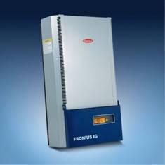
fig 3: Fronius IG with display
Battery bank
The batteries are added in the system to insure electric for night time, days with low power production or cloudy days. This is not a normal car battery because a car battery is made for high power in few seconds. The most cars start after this and 3-5% of the charge is used for turning the starter.
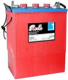
fig 4: Deep cycle battery from Surrette
Batteries for off grid systems are the same type as forklift and golf cars use. This type of batteries are called deep cycle batteries. Deep cycle means that it is possible to discharge the battery down to 20% of the charge. This is the maximum discharge. Manufactures has a general recommendation which is discharging down to 40%[3] . The batteries has voltage in the range 4-8v DC. The off-grid system has an operating level at 12-24v DC and the batteries have to be connected according the voltage. This is done by connecting the batteries in series to increase voltage. When the right system voltage is reach, the rest of the batteries are parallel connected. This all depends on the sizing of the bank and the battery setup. There are different kind of batteries design and this report well not go further with selection of batteries other than some general recommendations. The batteries have a shorter life span than the rest of the system and needs maintenance. Depending on the battery type and manufacture, there is a startup period where the capacity of the bank will go up and after some time degradation starts. It is important to follow the recommendations because batteries are expensive to buy in the right quality and if they are operated/not maintained after the recommendations, degradation could be complete in few years. Remember that a car battery is used 200-250 times per year and after 5-8 years it is replaced. After 4-6 years is hard to start the car in cold weather. The batteries for the off-grid system are constantly charge and discharge. They need to be taken care of.
Simulation of off grid system
To size the off-grid system, calculating the production and finally calculated the cost was a part of the assignment of this report. Therefore a simulation program was either to be programmed or an existing program adapted for calculations in this report.
After some investigations of different programs, a computer model with the name HOMER[4] was selected. It is a computer model first develop by National Renewable Energy Laboratory[5] and some years ago, distribution and supported was taken over by HOMER ENERGY. It is freeware currently and can be downloaded from their homepage.
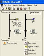
fig 5: Equipment overview
It has a focus on evaluating off and on-grid designs with renewable energy sources and has a sensitivity analysis built in. This gives opportunities to investigate change in demand which has a large impact on sizing a off grid system. HOMER has an hour to hour simulation and this gives possibilities to investigate how the battery bank status is and determine the sizing of the batteries. HOMER is build with an optimization focus and this means that the model tries to reduce cost of electricity. For this report some of the parameters need to be change to make the simulations for Greenland. The standard setting in HOMER for capacity shortage is 0%, because the model is suppose to cover all electric use and other users of the program typical has 20-60% renewable energy in the system and a generator as the main power source. This assumed not to be feasible for Greenland because of add cost and some adjustment of the model is needed to applied 100% renewable electric generation.
HOMER has a feature for cost calculation where an input for one size is given and HOMER use an linear regression to calculated price for other sizes. This should be used with care because typically there will be a rebate for buying large quantities or a bigger size is cheaper per unit. It is a good indicator but regressions outside the price range from the sales person or homepage should be used with care.
1
Electricity demand
To size the electricity production system for the house, the demand needs to be known. There is no measure data for the house so an estimate for the demand is going to be calculated. There are two key variables which influence sizing of the off grid system, average electric consumption and peak electric demand. The average electric usage is what the average is though the day. This is what the overall daily energy system should produce. The peak electric usage is what the battery bank and inverter should handle when a high load situation occur.
Demand curve
When a light is turn on there is a demand for electricity. In the same second as the receptacle is pressed, we expect to have power in the outlet. The power should be the right voltage and frequency. There is a net operator which forecast the demand and adjusts the power plants to meet the demand. There is a 24 hour forecast and minute to minute regulation of the grid demand/power production. This is adjusted so the ideal frequency is what the net sees. The ideal frequency is an indicator of no need for adjustment in the power production. If this is not meet (within a level), the power grid will have a fallout or burn a fuse. The systems operator can not adjust the demand but adjust the power production.
When a off grid installation is installed the owner becomes the system operator. The operator part is adjusting the demand curve with use of electrical items. For an average Danish household the yearly electric demand is in the range of 4000kWh for a house without electric heating and for a house with electric heating, between 9000 and 11000 kWh depending on the winter weather.
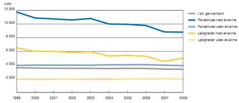
fig 6 - Danish electric demand average www.danskenergi.dk
Estimating services (Demand)
For the house on Greenland a demand has been estimated for a normal house with a kitchen , 2 rooms , a bathroom , hallway and a small shed . The estimate is made based on the services a house needs. There are made two different estimates of energy demand, one with normal appliances and one with energy efficient appliances.
Consumption with normal appliances
In Fejl! Henvisningskilde ikke fundet. the consumption is estimated and calculated. The focus has been to get all the normal services that the house users needs, find the standard appliances, estimate the usage and calculated the daily consumption.
Table 1 - Consumption with normal appliances
|
|
Services /appliances |
Power of the appliances [w] |
Operating time per day [minutes] |
Daily consumption [kWh] |
Link to appliances |
|
Kitchen |
Oven |
2000 |
30 |
1,00 |
|
|
|
Cooking plate |
3000 |
20 |
1,00 |
|
|
|
Kettle |
2200 |
3 |
0,11 |
|
|
|
Coffee maker |
1520 |
14 |
0,35 |
|
|
|
Refrigerator |
77 |
290 |
0,37 |
|
|
|
Mixer |
300 |
10 |
0,05 |
|
|
|
Microwave oven |
800 |
5 |
0,07 |
|
|
|
Light |
240 |
240 |
0,96 |
|
|
Hall way |
Light |
180 |
240 |
0,72 |
|
|
|
Frezer |
85 |
540 |
0,77 |
|
|
|
Waterheater |
3600 |
60 |
3,60 |
|
|
Bathroom |
Light |
180 |
60 |
0,18 |
|
|
|
Electric floor heating |
150 |
300 |
0,75 |
|
|
|
Washing machine |
- |
- |
0,57 |
|
|
|
Shaver |
50 |
5 |
0,00 |
|
|
Room 1 |
Computer |
65 |
240 |
0,26 |
|
|
|
Wifi Router |
12 |
1440 |
0,29 |
|
|
|
Link to satellite |
38 |
1440 |
0,91 |
|
|
|
Light |
120 |
240 |
0,48 |
|
|
Room 2 |
Light |
120 |
240 |
0,48 |
|
|
Shed |
Light |
120 |
120 |
0,24 |
|
|
|
Drill |
400 |
30 |
0,20 |
|
|
|
Powersaw |
400 |
10 |
0,07 |
|
|
|
Sum |
15657 |
5577 |
13,43 |
|
|
kWh
per day 13,43 |
kWh/year 4927,5 |
||||
The kitchen has standard appliances and is assume that both the oven and cooking plates is use for daily cooking. This is not true when the dish is spaghetti and meat sauce but in the weekends it is used. This is where the estimating factor influents the system designs and the actual usage could differ significantly.
The hallway has a water heater which makes the domestic hot water for the house and it is 26% of the daily consumption. This is also an appliances which needs to be controlled, because the load is significant and influents the inventor sizing significantly.
Room 1 has two 24 hours consumption, a wireless router and a satellite internet link. Both are on due to comfort. It takes time to track the satellite if it has been turn off and the route has an initialization time.
The shed is calculated with a daily usage
of the drill and power saw. The shed can
have a varying load and the most import thing is the peak demand for this room.
This means that the power of the appliances is the most important number.
Load/peak curve for consumption with normal appliances.
Sizing of the inventor and battery system depends on the load. The estimated of the load situation has been made in Appendix 2: and the result can be seen in fig 7. It is based on which time range of the 24 hours that the appliances could be on and if the appliance has a shift in demand. An example on a shift appliance could be the water heater. Morning shower is between 6:30 and 8:00. So the water heater is likely to start between 7 and 8:30 because the heating of water first starts when some of the hot water has been used. Depending on the length of the shower, the heater will be on shorter or longer time. fig 7 has both the number of items on and the load. This is because the user of the house needs to be aware that even if, a few items is on, there can still be a large peak load (water heater, oven, etc).
It I seen that the peak load is at 18:00 and it is 7, 5 kW. This needs to be lowered with a factor because this figure is made for each hour and to estimate the right peak value, it needs to be based on minutes or even seconds. It is unlikely that all the items estimated to be use in the same hour is on simultaneous. So the value is lowered with 25%, down to 5,5kw. The 25% is an assumption made.
The load/peak curve influents the system cost because it is optimal with a load when the energy production occur. That is where the simulation program needs an hour based load profile to calculate the battery sizing and the values from the load/peak curve is used as an input.
fig 7 - Load/peak curve for consumption with normal appliances.
Consumption with efficient appliances and change of heat input
In Table 2 , a new consumption with energy efficient appliances has been calculated. All the services from Fejl! Henvisningskilde ikke fundet. have been kept but some of the appliances have been improved. The normal appliances already have some energy efficient appliances, compare with standard appliances. It is hard to find appliances which are not A rate in energy efficient usage because the Danish Electricity Saving Trust has done a large amount of work to promote those appliances and they are the cheapest appliances to buy today.
Table 2- Consumption with efficient appliances and change of heat input
|
Services /appliances |
Power of the appliances [w] |
Operating time per day [minutes] |
Daily consumption [kWh] |
Link to appliances |
|
|
Kitchen |
Oven |
2000 |
30 |
1,00 |
|
|
|
Cooking plate |
3000 |
20 |
1,00 |
|
|
|
Kettle |
2200 |
3 |
0,11 |
|
|
|
Coffee maker |
1520 |
14 |
0,35 |
|
|
|
Refrigerator |
77 |
290 |
0,37 |
|
|
|
Mixer |
300 |
10 |
0,05 |
|
|
|
Microwave oven |
800 |
5 |
0,07 |
|
|
|
Light |
42 |
240 |
0,17 |
|
|
Hall way |
Light |
14 |
240 |
0,06 |
|
|
|
Frezer |
85 |
540 |
0,77 |
|
|
|
Waterheater |
3600 |
60 |
0,00 |
|
|
Bathroom |
Light |
28 |
60 |
0,03 |
|
|
|
Electric floor heating |
150 |
300 |
0,00 |
|
|
|
Washing machine |
- |
- |
0,57 |
|
|
|
Shaver |
50 |
5 |
0,00 |
|
|
Room 1 |
Computer |
65 |
240 |
0,26 |
|
|
|
Wifi Router |
12 |
260 |
0,05 |
|
|
|
Link to satellite |
38 |
260 |
0,16 |
|
|
|
Light |
10 |
240 |
0,04 |
|
|
Room 2 |
Light |
14 |
240 |
0,06 |
|
|
Shed |
Light |
14 |
120 |
0,03 |
|
|
|
Drill |
400 |
30 |
0,20 |
|
|
|
Powersaw |
400 |
10 |
0,07 |
|
|
|
Sum |
14819 |
3217 |
5,41 |
|
|
kWh per day 5,42 |
kWh/year 2007,5 |
||||
For all the rooms the incandescent light has been switch to LED light. It has the same light but with much lower energy consumption. With the same light, LED use 7 watt compare to a normal 60 watt light bulb.
The kitchen appliances is still the A rate appliances. No major change.
In the hall way, the water heater has been change to a gas fire heater. This is a major reduction in power consumption. This means that the house needs a gas heater and supply gas from a gas cylinder. It needs further investigation if it is feasible on Greenland.
In the bathroom the electric floor heating has been turn off. This is services which adds appreciation in the morning and should maybe be turn on again. The always on wifi router and satellite link in room 1 one has been equip with a main on/off and the user needs to start it up 10 minutes before use.
The total savings with this minor change in heating , investment in LED lights and change of habits add up to 8kWh in Table 3. This is large reduction in daily electric consumption.
Table 3 - Savings
|
Services /appliances |
Daily Savings [kWh] |
|
LED light |
2,68 |
|
Waterheater |
3,60 |
|
Electric floor heating |
0,98 |
|
Wi-Fi/ satellite |
0,75 |
|
Sum |
8,02 |
Load/peak curve with efficient appliances and change of heat input
In fig 8 is shown that there is a significant change in load and a minor change in peak load. From 8 to 11 am the heating of water is gone and all day the Wi-Fi/ satellite equipment is removed from the base load. The peak load is reduced with 400watt and is still 7,1 kW. With the 25% reduction because of the applicens is not on at the same time, it gives a peak load for the inventor at 5,3kW. It is a factor with would be ideal to lower, because of reduction of inventor cost.
fig 8 - Peak load with normal and efficient appliances
Simulation input from services loads.
From the two load situations the daily load and peak load value is use in the simulation software. The consumption is estimated from calculations but in comparison with average Danish electricity consumption level at 4000kWh, 4902 kWh is feasible. The focus on efficient appliances gave a saving of 60% consumption and it is possible to reduce the consumption more. A 60 % reduction in consumption yearly without lowering the services level is very good and it should be possible to lower it 50% more, down to a 1:4 of the original consumption.
Table 4 – Services loads
|
|
Normal appliances |
Efficient appliances |
Savings |
|
Daily consumption [kWh] |
13,43 |
5,41 |
60% |
|
Yearly consumption [kWh] |
4902 |
1975 |
60% |
|
Peak load [kW] |
5,5 |
5,3 |
4% |
2
Method
Preparation of input data
In order to use HOMER and other simulation/calculation programs a set of input data has to be defined to make the simulation work.
Weather data
The provided weather data are “TRY” files which among other things contains data about mean hourly global irradiance, in W/m² and wind speed, in m/s. This data are extracted to separate files via Excel. From which fig 9 and fig 10 are made. – For comparison weather data from Copenhagen is added.
fig 9: Average "Mean hourly global
irradiance" in W/m2 for each month for each of the three
Greenlandic cities
Uummannaq and Nuuk are the two cities with highest averages mean hourly global irradiance according to fig 9. It is also seen that in jan, nov and dec there is almost no global irradiance for the 3 cities.
fig 10: Average "Wind speed" in
m/s for each month for each of the three Greenlandic cities
From fig 10 Nuuk are the city with the highest average wind speed and the two other cities are lower then Nuuk.
In HOMER the solar radiation is given as daily radiation kWh per square metre per day as in fig 11.
fig 11: Daily radiation in kWh/m2/d
for each of the cities
In Appendix 1: Weather data tables with data figures 2 to 4.
General simulation inputs
The general simulation inputs are used in all simulations. These inputs are placed in HOMER and can be activated/de activated when need but they are stored inside HOMER. The following inputs is based in the information found in Appendix 5:
Table 5: Equipment size and prices
|
Item |
Size |
Capital
(kr) |
Replacement
cost ($/year) |
Operation
and maintenance cost (kr/year) |
Size (kW) |
Quantities
considered |
Life time |
|
PV |
1 |
kr 8.240 |
kr 7.240 |
kr - |
0-30 |
- |
20 years |
|
Inverter |
1 |
kr 5.060 |
kr 4.060 |
kr - |
0-6 |
- |
15 years |
|
Battery |
1156 Ah |
kr 5.245 |
kr 4.745 |
kr 100 |
- |
0-50 |
12~20 years |
To optimize computational time a linear size/quantities formula is used to increase speed and find the solution space. As the size is getting narrower HOMER starts to spend more calculation time on each solution and the refine hour to hour status are calculated. A typical simulation has between 2000 and 7000 part simulations and each simulation starts over when the sensitivity analyze function is used. 100 simulations can be calculated per second with 5 sensitivities in the load curve it gives a calculation time between 3 and 5 minutes. This is fast compare with a 60 minute time step in each simulation for all year. This is also an issue when the simulation is only for 4 months in the year because HOMER stills calculates for the complete year, even if the load and renewable source are set to zero.

fig 12: Example on step vs. array size
Load input
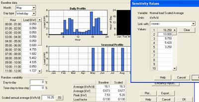
fig 13: Input window for loads
The demand from section 2 is used in the loads window for May to August month. That is the Baseline and the scaled annual average is where the different loads are used as inputs. They can be seen in. HOMER has a random variability function with a day to day and step to step change. In the simulations for this reports those values has been zero because a refine hour to hour curve has been made.
Table 6: Loads used for simulations

Grid extension
This off-grid system is compare with the price of an extension. Normally the cable for a grid connection is dig down. On Greenland this it made on another method because of rocks. First a metal profile is attached to the rocks and a cable with a large cross sectional area is placed in the metal profile. The cable is then attach to the profile with small robs and then the metal profile is welded together[6].
It is assumed to be in the range of 50.000 to 250.000 kr/km and this is used as an input in Homer.
Table 7: Price of grid extension
|
Sensitivity |
Price per km cable inc. connection to electricity meter |
|
1 |
50.000 kr. |
|
2 |
100.000 kr. |
|
3 |
150.000 kr. |
|
4 |
200.000 kr. |
|
5 |
250.000 kr. |
HOMER uses the price of electrify to calculated the total cost for the off-grid and grid extension. The power company in Greenland has a pricelist online[7] and the current price per kWh is used as an input.
Table 8: Electricity price on Greenland
|
City |
Price per kWh inc. tax |
|
Nuuk |
1.48 kr. |
|
Uummannaq |
2.82 kr. |
|
Sisimiut |
2.23 kr. |
Constraints
HOMER has an input for system constants. Almost all of them can be set to zero because they are options for generator operation strategies. There is one setting which is the Maximum Annual Capacity Shortage which needs to be change. This is a constraints is how many of the hours where there is a shortage is approved. This is normally set to 0% but with a small off grid installation the price of the installation drops if some unmet demand is approved. Because HOMER is an optimization model it seems to use the constraints as stop criteria for optimization. So the shortage has been set to 10%. This does that HOMER calculated after the demand and do not use the Maximum Annual Capacity Shortage as stop criteria. This is parameter which could be improved in HOMER.
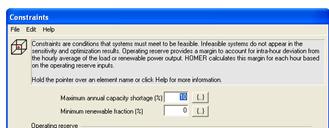
fig 14: HOMER constraints
Off-grid system with a household turbine
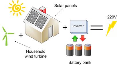
fig 15: Off-grid system with PV and household wind turbine
The weather data for the tree cites in Greenland includes measurements for wind speed. HOMER has an option for adding a household wind turbine. A wind turbine is cheaper per kW installed capacity and mostly the kWh is also lower compared to PV. Wind turbines typically work at night and this is a problem in an off grid system because the energy needs storage and batteries are by no means cheap. It could be a supplement for the solar. The size of wind turbines for this off-grid system is in the range of 0.5 to 2.5kW which is in a prince range of 13.800 to 45.2000kr.
Table 9: Household Wind turbines
|
Name |
Rate
output |
Total
height |
Price |
www |
|
BWC XL.1 |
1000 W DC |
9 m |
kr
13.800 |
|
|
SW Whisper
500 |
3000 W DC |
16 m |
kr
42.500 |
For this report the wind turbine is assume to be a block box which gives an output. There are different considerations which should be done when a turbine is selected, especially when a place like Greenland is considered. This is dude to icing of the blades and spare parts. Compare with the PV panels the small turbines are known for need of maintenances.
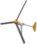
fig 16: Bergey XL 1
3
Results
Simulations for Nuuk from May to august month
Table
10: Simulation results for Nuuk in the
period May to August with up to 10 % unmet demand
|
PV |
Battery |
Converter |
Unmet Load Fraction |
Cost of electricity |
Total NPC |
|
|
kWh/d |
kW |
Quantities |
kW |
Kr/kWh |
Kr. |
|
|
16 |
13.07 |
24 |
5.0 |
0.08 |
5.93 |
637.484 |
|
13 |
10.46 |
20 |
3.0 |
0.08 |
5.84 |
508.925 |
|
9.75 |
8.37 |
12 |
3.0 |
0.08 |
5.80 |
378.119 |
|
5.42 (Eff) |
4.28 |
12 |
1.8 |
0.06 |
6.60 |
244.789 |
|
3.25 |
2.74 |
5 |
1.0 |
0.07 |
6.02 |
132.883 |
Focus on the 13kWh load.
The results are seen in Table 10 for Nuuk. For the normal load situation with 13kWh and a peak load at 5,3kW the total net present cost (NPC)[8] is 508.925kr. This is a big investment for four months of use per year and it is seen that the solar panels is a 10.5 kW array.
Table 11: PV production for 13kWh load at
Nuuk in the period May to August
|
Quantity |
Value |
Units |
|
Rated capacity |
10.5 |
kW |
|
Mean output |
0.69 |
kW |
|
Mean output |
16.6 |
kWh/day |
|
Capacity factor |
6.61 |
% |
|
Total production |
6059 |
kWh/yr |
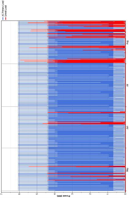
The solar panels are 323.000kr (80%) for the capital cost and their performance should be analyzed. As a rule of thumb a normal annual output for 1kW in the range 800-1200kWh. This simulation is only for the four best solar months, so the output of 577 kWh per kW panel seems likely. The complete system price which HOMER calculates has been checked with IEA SOLAR[9] average installed system prices which are 46,5kr/W peak power. This gives a system price at 488.000kr. So the price is in the right range. The next things are sizing of the system. Because of the battery’s it when the batteries are empty that the system price starts to increase because when the house is running at batteries for a longer time, they need to be charge when the sun is shining and this adds more solar panels to the PV system. An overview of the load and unmet demand can be found in Appendix 3: . A period on this graph is selected out for further analyze.
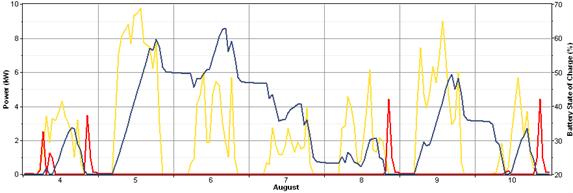
![]()
fig 17: PV output, unmet load and battery
state– 13kWh in the period 4 to 10 August
Fig 17 shows the period between the 4 and 10 august. It is seen that in the period 5-7 august there is no unmet load but the state of the battery bank goes from 50 % to 20% at night. There is generated solar power each day but it is decreasing in the period from a daily output at 8kW down to 2 KW. The 8 of august there is an unmet demand in the period 19:00 unto morning of the 9 august. This can be seen in fig 18 which is a plot of the 24 hours.
So the question is what does it means for the user of the house and is it okay when the owner just pay close to half a million kr. for the system?
As
seen on the figure there is actually both excess electric that day and power
most of the day. It is just after
cooking where there is high load for 2-3 hours. If the users of the house had a
look on the battery controller they could for see that the battery was running
out of power and could instead had grill or had cold food for dinner. This
would have lowered the power consumption and there would have been light for reading
or satellite internet. So buying more batteries and PV to charge them is an
expensive option, compare to just leaving the oven off that night. In general
renewable off grid system is expensive and a little awareness makes the
off-grid system for a 13kWh load per day a perfect option compare which is
comparable to a grid connection.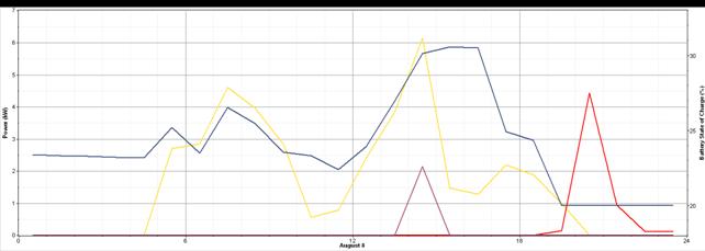
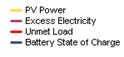
fig 18: PV output , excess power, unmet
load and battery state– 13kWh the 8 of August
Focus on the 5,42kWh load.
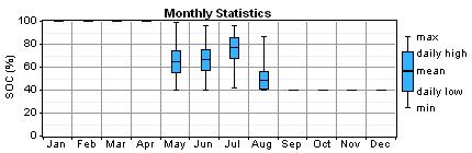
Compare with the system for a 13kWh load the daily consumption is the half and the cost is actually the half. The remarkable change is the size of the PV system is 40 % of the 13 kWh but the battery bank is the half. This indicated that the load though most of the days can be handle with the PV panels and some of the battery capacity. fig 19 shows the state of battery bank and it has a little deep in the start of august, otherwise is keeps is it above 70%. This means that for half of the cost of a 13kWh system there is a better load handling. It is possible to state that this system is equal with a grid connection.
fig 19: Battery bank - 5kWh Nuuk
Grid extension results Nuuk
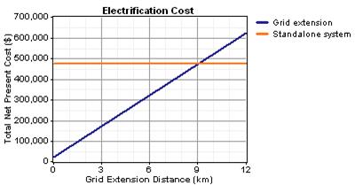
Fig 20 shows the distance as a function of the cost per km to install the grid connection. As it is seen on the graph the 13kWh system can have a grid connection installed from almost 10 km away if the installation cost is 50.000kr. per km. It is seen that that distance falls rapidly when the price per km is add 50.000kr in each simulation. Already with a cost of 150.000kr which should be a normal price to pay, the 13kWh is feasible at 3.3 km. If a house has an idea about an off-grid system, it is properly above 3.3 km away.
fig 20: Grid extension Nuuk
Simulations for Sisimiut from May to august month
fig 21 show the simulation results from Sisimiut. Compare to Nuuk it is in the same price range and quantities. This is compare with a little lower measured mean hourly global irradiance. This gives a higher cost of produced electricity.
|
PV |
Battery |
Converter |
Unmet Load Fraction |
Cost of electricity |
Total NPC |
|
|
kWh/d |
kW |
Quantities |
kW |
Kr/kWh |
Kr. |
|
|
16 |
13.07 |
24 |
8.0 |
0.10 |
6.26 |
660.736 |
|
13 |
10.46 |
20 |
7.0 |
0.10 |
6.31 |
539.922 |
|
9.75 |
8.37 |
14 |
5.0 |
0.09 |
6.33 |
410.426 |
|
5.42 (Eff) |
4.28 |
12 |
3.0 |
0.08 |
6.96 |
254.087 |
|
3.25 |
2.74 |
5 |
1.8 |
0.09 |
6.42 |
139.089 |
fig 21: Simulation results for Sisimiut in
the period May to August with up to 10 % unmet demand
Simulations for Uummannaq from May to august month
fig 22 shows the results for Uummannaq. The total NPC is lower for each load situation compare with Nuuk and Sisimuit. The battery numbers is lower than the two other cities. This reducers’ the cost significantly and in fig 23 shows that in the higher loads Uummannaq an advantage
|
PV |
Battery |
Converter |
Unmet Load Fraction |
Cost of electricity |
Total NPC |
|
|
kWh/d |
kW |
Quantities |
kW |
Kr/kWh |
Kr. |
|
|
16 |
10.46 |
12 |
3.0 |
0.10 |
4.20 |
441.652 |
|
13 |
6.69 |
16 |
3.0 |
0.10 |
4.21 |
360.924 |
|
9.75 |
5.36 |
12 |
3.0 |
0.08 |
4.39 |
286.618 |
|
5.42 (Eff) |
3.43 |
4 |
1.8 |
0.09 |
4.20 |
151.488 |
|
3.25 |
2.19 |
2 |
1.0 |
0.09 |
4.23 |
90.988 |
fig 22: Simulation results for Uummannaq in the period May to August with up to 10 % unmet demand
fig 23: Comparison for 5
different loads in the tree cities
Simulations for Nuuk, from May to august month, with a household wind turbine
Homer has been given the weather data and the possibility to add a 3kW turbine in Table 12. HOMER chooses to operate the turbine and it is seen that the size of the PV array is almost half and the same is the number of batteries, compare with Nuuk with only a PV system. This shows there is synergy between the two renewable power generation sources. It should also be seen that HOMER does not have a pure wind/battery solution as a option. This indicates that PV/Wind is a optimal solution and it is seen that the capital cost has been reducere significant compare to the PV solution.
Table 12: Simulation results for Nuuk in the period May to August with up to 10 % unmet demand and 3 kW turbine
|
load |
PV |
Turbine |
Battery |
Converter |
Converter |
Unmet Load Fraction |
Cost of electricity |
Capital cost |
|
kWh/d |
kW |
Quantities |
Quantities |
kW |
kW |
Kr/kWh |
Kr. |
|
|
16.00 |
8.37 |
1.00 |
12 |
3.0 |
3.0 |
0.10 |
4.32 |
378.54 |
|
13.00 |
5.36 |
1.00 |
12 |
3.0 |
3.0 |
0.09 |
4.22 |
287.05 |
|
9.75 |
4.28 |
1.00 |
5 |
3.0 |
3.0 |
0.09 |
4.18 |
217.80 |
|
5.42 |
1.12 |
1.00 |
4 |
1.0 |
1.0 |
0.10 |
4.27 |
104.92 |
|
3.25 |
0.23 |
1.00 |
2 |
1.0 |
1.0 |
0.10 |
4.82 |
62.83 |
fig 24 show comparison of the capital cost of the 3 solutions and it is seen that the cost is has the biggest decrease for higher loads. When the load is under 6 kWh daily the different between the two size turbines becomes insignificant. Stile there is an advantage to combine PV and a small turbine.
fig 24: Comparison between
PV and 2 turbine size for Nuuk
Simulations for Sismumt, from May to august month, with a household wind turbine
It is seen in fig 25 that for Sismumt that PV is the best option. This is due to weather conditions in Sismumt. The wind speed in May to August in Sismumt is almost below the thresholds of a household wind turbine and this condition makes PV attractive.
fig 25: Comparison between
PV and 2 turbine size for Sismumt
Simulations for Uummannaq, from May to august month, with a household wind turbine
fig 26 shows that same picture as fig 25, Uummannaq has to low wind to make PV/Wind attractive and PV is the most attractive solution.
fig 26: Comparison between
PV and 2 turbine size for Uummannaq
Result
for Breakeven grid distance
Table 13 shows the breakeven distance for different load and the breakeven distance are calculated for five different prices for each city. Within the city column tree different solutions are used and the minimal distance is marked with a bold type. The cost of the individual system can be seen in the report.
Table 13: Breakeven grid distance
|
Load |
Grid extension cost Kr/km |
Nuuk |
Sismumt |
Uummannaq |
||||||
|
kWh Daily |
PV |
PV+1kW Turbine |
PV+3kW turbine |
PV |
PV+1kW Turbine |
PV+3kW turbine |
PV |
PV+1kW Turbine |
PV+3kW turbine |
|
|
16 |
kr 50.000 |
12.17 |
10.53 |
8.52 |
8.01 |
10.97 |
10.15 |
7.74 |
8.20 |
8.32 |
|
|
kr 100.000 |
6.09 |
5.26 |
4.26 |
4.00 |
5.48 |
5.08 |
3.87 |
4.10 |
4.16 |
|
|
kr 150.000 |
4.06 |
3.51 |
2.84 |
2.67 |
3.66 |
3.38 |
2.58 |
2.73 |
2.77 |
|
|
kr 200.000 |
3.04 |
2.63 |
2.13 |
2.00 |
2.74 |
2.54 |
1.93 |
2.05 |
2.08 |
|
|
kr 250.000 |
2.43 |
2.11 |
1.70 |
1.60 |
2.19 |
2.03 |
1.55 |
1.64 |
1.66 |
|
13 |
kr 50.000 |
9.71 |
8.38 |
6.80 |
6.57 |
8.90 |
8.40 |
6.33 |
6.41 |
7.03 |
|
|
kr 100.000 |
4.86 |
4.19 |
3.40 |
3.28 |
4.45 |
4.20 |
3.16 |
3.20 |
3.52 |
|
|
kr 150.000 |
3.24 |
2.79 |
2.27 |
2.19 |
2.97 |
2.80 |
2.11 |
2.14 |
2.34 |
|
|
kr 200.000 |
2.43 |
2.10 |
1.70 |
1.64 |
2.22 |
2.10 |
1.58 |
1.60 |
1.76 |
|
|
kr 250.000 |
1.94 |
1.68 |
1.36 |
1.31 |
1.78 |
1.68 |
1.27 |
1.28 |
1.41 |
|
9.75 |
kr 50.000 |
7.21 |
6.96 |
5.09 |
5.03 |
6.78 |
6.74 |
5.06 |
5.45 |
5.43 |
|
|
kr 100.000 |
3.61 |
3.48 |
2.54 |
2.52 |
3.39 |
3.37 |
2.53 |
2.73 |
2.71 |
|
|
kr 150.000 |
2.40 |
2.32 |
1.70 |
1.68 |
2.26 |
2.25 |
1.69 |
1.82 |
1.81 |
|
|
kr 200.000 |
1.80 |
1.74 |
1.27 |
1.26 |
1.70 |
1.69 |
1.27 |
1.36 |
1.36 |
|
|
kr 250.000 |
1.44 |
1.39 |
1.02 |
1.01 |
1.36 |
1.35 |
1.01 |
1.09 |
1.09 |
|
5.42 |
kr 50.000 |
4.70 |
3.54 |
2.84 |
3.32 |
4.02 |
3.86 |
2.66 |
3.16 |
3.45 |
|
|
kr 100.000 |
2.35 |
1.77 |
1.42 |
1.66 |
2.01 |
1.93 |
1.33 |
1.58 |
1.72 |
|
|
kr 150.000 |
1.57 |
1.18 |
0.95 |
1.11 |
1.34 |
1.29 |
0.89 |
1.05 |
1.15 |
|
|
kr 200.000 |
1.18 |
0.88 |
0.71 |
0.83 |
1.01 |
0.97 |
0.66 |
0.79 |
0.86 |
|
|
kr 250.000 |
0.94 |
0.71 |
0.57 |
0.66 |
0.80 |
0.77 |
0.53 |
0.63 |
0.69 |
|
3.25 |
kr 50.000 |
2.54 |
2.17 |
1.95 |
1.72 |
2.58 |
2.70 |
1.60 |
2.08 |
2.41 |
|
|
kr 100.000 |
1.27 |
1.09 |
0.98 |
0.86 |
1.29 |
1.35 |
0.80 |
1.04 |
1.21 |
|
|
kr 150.000 |
0.85 |
0.72 |
0.65 |
0.57 |
0.86 |
0.90 |
0.53 |
0.69 |
0.80 |
|
|
kr 200.000 |
0.64 |
0.54 |
0.49 |
0.43 |
0.64 |
0.68 |
0.40 |
0.52 |
0.60 |
|
|
kr 250.000 |
0.51 |
0.43 |
0.39 |
0.34 |
0.52 |
0.54 |
0.32 |
0.42 |
0.48 |
4
Discussion
The simulation has been made with the weather data for one year and it the conclusion is based on this weather data. If there is weather data available for more years, it is an option to simulated for those years also and verify the systems sizing is accurate for more weather conditions.
The house has been equipped with the different appliances that there is available in a standard house. This is assumption and compare with the usage period from May to August, this house should perhaps has been equipped like a summer house and some of the appliances should have been removed.
The demand has been made artificially and it will be different in the real world. It has also been shown that it is possibly to lower the demand in half and even more is to be expected. After all the simulations is made, it is shown more exploration of lowering the energy demand is the best option to lower the price of the off grid system.
Adding the wind turbine has shown results that wind turbines is not necessarily a good option in the period of May to August but if the usage period of the house is extend initial simulations has shown that it is a necessary to have a wind turbine. The means that is the off grid system usage period is extern some months in each end of the May to August period, it will have problems with generating enough electricity.
5
Conclusion
Off grid systems have been an option for years. The technology has to an extern been proven and it is know a full-grown option to a grid extension. The cost of the off grid system has been calculated and compare with a grid extension a series of analyze has been made. Those analyze is based on measured weather data for 3 cites in Greenland.
The processed weather data has been a signification factor to calculations of the right size system. When that quality of weather data is available it should be use to optimized the initial system and when the system is installed the same weather should existed. This means that there should be no new obstacles which is shadowing for the PV and possible wind turbine.
Calculating the electric load and making a demand curve has been a challenge which has shown the need for real world measurements. This issue was work out by calculating a daily load and making a demand curve. Those calculations is based on information about electrical appliances and based on changing out some of the equipment out with more efficient appliances and switching from electrical heating to gas heating the electrical load was lowered into the half.
HOMER has shown to be a fast and comprehensive optimization program. There has been used time to learn the program and make the inputs right. This has been a great method to get a knowledge of the influents of the different factors which impacts a off-grid system and from a initial time step at 5 hours to make fast calculations, down to 60 minutes when the simulations for the report was made. This gives an opportunity to follow responses for all system states and from this numbers, see the battery state and which time the battery is in used and how low the charge is. This gives a great understanding of the system.
The simulations have been focused on PV with a battery bank and it has given broad range of results for different load situations and it has been shown that the local weather in each city has large influents on the electric production. For the same off-grid system there is a different of 2 km for the breakeven distance grid connection. This is the differences between placing the off-grid system in Uummannaq instead of Nuuk.
Adding wind turbines as option had an unexpected solution space. The initial assumption has that adding a small turbine was lowering the cost of the off-grid system. It has true for Nuuk in all load situations but for Sismumt and Uummannaq it was adding extra cost to the system and the optimal solution was a pure PV system. This shows that simulation with real weather data gives the best solution and it is not necessarily a good idea to combine PV and wind when cost is the driver. In this context there should be sad, that the wind turbine didn’t help in the unmet load faction. It was better with the PV only system.
The main conclusion is that a daily load of 5.5 kWh gives, even with the lowest price of the grid extension, a maximal breakeven distance is 3.32km for all three cities. This is seems to be a short distance on Greenland and this is without lowering services level.
6
Recommendations
·
This
report has shown a basis project and some existing equipment which could be
used on Greenland but the equipment should be insure to be rugged and suitable
for remote communities. Those communities does not have the expertise to repair
this type of installation
·
A
pilot or proof of concept should be implemented in Nuuk. It is properly the
easiest citie to find some expertise and the pilot system should withstand one
summer and one average winter before it is deplored into remote cities
·
A
guide book for buying and minor repairs should be made, to insure operation of
the isolated system.
·
This
recommendations should insure that a positive, well documented track record
well make off-grid installations a success on Greenland and in that way
implement 100% renewable energy which is a equal panther to grid extensions and
hopefully , the preferred solution!
7
Appendices
Appendix 1: Weather data
From the provided weather data files both for Greenland (TRY) and Copenhagen (DRY) the following tables are made to summarize the information:
Table 14: Weather data from NUUK
|
|
Gh
[W/m2] |
Ws
[m/s] |
kWh/m2/d |
||
|
|
average |
max |
average |
max |
HOMER |
|
jan |
6.53 |
142 |
7.24 |
22.30 |
0.157 |
|
feb |
30.50 |
320 |
6.98 |
18.70 |
0.732 |
|
mar |
94.79 |
561 |
6.79 |
20.00 |
2.275 |
|
apr |
152.65 |
669 |
5.93 |
21.00 |
3.664 |
|
may |
199.49 |
773 |
6.05 |
20.20 |
4.788 |
|
jun |
220.74 |
840 |
5.16 |
24.10 |
5.298 |
|
jul |
251.05 |
787 |
4.77 |
20.50 |
6.025 |
|
aug |
141.12 |
695 |
5.49 |
23.20 |
3.387 |
|
sep |
75.49 |
602 |
5.38 |
27.90 |
1.812 |
|
oct |
42.45 |
364 |
5.04 |
17.50 |
1.019 |
|
nov |
10.62 |
173 |
6.34 |
24.70 |
0.255 |
|
dec |
2.33 |
49 |
6.71 |
20.20 |
0.056 |
Table 15: Weather data from SISIMIUT
|
|
Gh
[W/m2] |
Ws
[m/s] |
kWh/m2/d |
||
|
|
average |
max |
average |
max |
HOMER |
|
jan |
2.58 |
66 |
3.86 |
13.90 |
0.062 |
|
feb |
23.58 |
260 |
3.57 |
16.60 |
0.566 |
|
mar |
91.78 |
459 |
3.33 |
16.50 |
2.203 |
|
apr |
146.96 |
656 |
3.10 |
19.00 |
3.527 |
|
may |
210.05 |
716 |
3.56 |
15.80 |
5.041 |
|
jun |
200.89 |
752 |
3.19 |
18.70 |
4.821 |
|
jul |
212.75 |
739 |
2.49 |
13.10 |
5.106 |
|
aug |
124.53 |
642 |
3.04 |
18.10 |
2.989 |
|
sep |
70.77 |
460 |
2.83 |
18.30 |
1.699 |
|
oct |
29.66 |
313 |
2.73 |
14.80 |
0.712 |
|
nov |
6.42 |
151 |
4.26 |
18.90 |
0.154 |
|
dec |
0.46 |
20 |
6.73 |
26.30 |
0.011 |
Table 16: Weather data from UUMMANNAQ
|
|
Gh
[W/m2] |
Ws
[m/s] |
kWh/m2/d |
||
|
|
average |
max |
average |
max |
HOMER |
|
jan |
0.34 |
16 |
4.59 |
18.40 |
0.008 |
|
feb |
16.58 |
295 |
3.92 |
13.60 |
0.398 |
|
mar |
95.29 |
519 |
1.62 |
17.10 |
2.287 |
|
apr |
172.47 |
591 |
2.39 |
10.80 |
4.139 |
|
may |
247.38 |
754 |
3.30 |
13.10 |
5.937 |
|
jun |
281.66 |
861 |
3.58 |
18.00 |
6.760 |
|
jul |
204.68 |
640 |
3.00 |
12.90 |
4.912 |
|
aug |
145.56 |
569 |
2.84 |
11.30 |
3.494 |
|
sep |
74.90 |
493 |
4.18 |
15.00 |
1.798 |
|
oct |
22.61 |
250 |
3.97 |
14.30 |
0.543 |
|
nov |
1.82 |
62 |
6.14 |
19.50 |
0.044 |
|
dec |
0.27 |
2 |
4.94 |
12.80 |
0.006 |
Table 17: Weather data from COPENHAGEN
|
|
Gh
[W/m2] |
Ws
[m/s] |
kWh/m2/d |
||
|
|
average |
max |
average |
max |
HOMER |
|
jan |
40.00 |
794 |
4.99 |
19.00 |
0.960 |
|
feb |
66.66 |
866 |
4.43 |
16.00 |
1.600 |
|
mar |
96.54 |
1038 |
4.84 |
18.00 |
2.317 |
|
apr |
154.40 |
1015 |
4.55 |
17.00 |
3.706 |
|
may |
208.63 |
996 |
4.10 |
15.10 |
5.007 |
|
jun |
188.64 |
898 |
3.79 |
13.30 |
4.527 |
|
jul |
174.59 |
918 |
3.87 |
13.40 |
4.190 |
|
aug |
164.06 |
916 |
3.53 |
15.00 |
3.937 |
|
sep |
120.51 |
867 |
4.37 |
17.50 |
2.892 |
|
oct |
75.59 |
833 |
4.54 |
17.00 |
1.814 |
|
nov |
43.93 |
820 |
4.53 |
20.70 |
1.054 |
|
dec |
25.37 |
650 |
4.90 |
18.70 |
0.609 |
Appendix 2: Demand
Appendix 3: Nuuk
Appendix 4: System Report - Nuuk_maj_august
Sensitivity case
|
|
Normal load Scaled Average: |
13 |
kWh/d |
|
|
Grid Extension Capital Cost: |
50,000 |
$/km |
System architecture
|
PV Array |
10.5 kW |
|
Battery |
16 Surrette 4KS25P |
|
Inverter |
3 kW |
|
Rectifier |
3 kW |
Cost summary
|
Total net present cost |
$
475,286 |
|
Levelized cost of energy |
$ 5.551/kWh |
|
Operating cost |
$
2,736/yr |
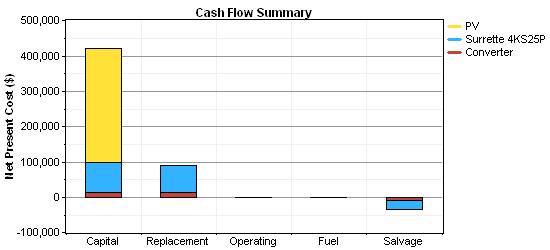
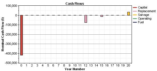
Net Present Costs
|
Component |
Capital |
Replacement |
O&M |
Fuel |
Salvage |
Total |
|
($) |
($) |
($) |
($) |
($) |
($) |
|
|
PV |
323,317 |
0 |
0 |
0 |
0 |
323,317 |
|
Surrette 4KS25P |
83,920 |
75,920 |
0 |
0 |
-25,307 |
134,533 |
|
Converter |
13,327 |
12,327 |
0 |
0 |
-8,218 |
17,435 |
|
System |
420,564 |
88,247 |
0 |
0 |
-33,524 |
475,286 |
Annualized Costs
|
Component |
Capital |
Replacement |
O&M |
Fuel |
Salvage |
Total |
|
($/yr) |
($/yr) |
($/yr) |
($/yr) |
($/yr) |
($/yr) |
|
|
PV |
16,166 |
0 |
0 |
0 |
0 |
16,166 |
|
Surrette 4KS25P |
4,196 |
3,796 |
0 |
0 |
-1,265 |
6,727 |
|
Converter |
666 |
616 |
0 |
0 |
-411 |
872 |
|
System |
21,028 |
4,412 |
0 |
0 |
-1,676 |
23,764 |
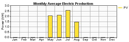
Electrical
|
Component |
Production |
Fraction |
|
(kWh/yr) |
||
|
PV array |
6,059 |
100% |
|
Total |
6,059 |
100% |
|
Load |
Consumption |
Fraction |
|
(kWh/yr) |
||
|
AC primary load |
4,281 |
100% |
|
Total |
4,281 |
100% |
|
Quantity |
Value |
Units |
|
Excess electricity |
933 |
kWh/yr |
|
Unmet load |
464 |
kWh/yr |
|
Capacity shortage |
464 |
kWh/yr |
|
Renewable fraction |
1.000 |
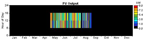
PV
|
Quantity |
Value |
Units |
|
Rated capacity |
10.5 |
kW |
|
Mean output |
0.692 |
kW |
|
Mean output |
16.6 |
kWh/d |
|
Capacity factor |
6.61 |
% |
|
Total production |
6,059 |
kWh/yr |
|
Quantity |
Value |
Units |
|
Minimum output |
0.00 |
kW |
|
Maximum output |
8.84 |
kW |
|
PV penetration |
128 |
% |
|
Hours of operation |
1,476 |
hr/yr |
|
Levelized cost |
2.67 |
$/kWh |
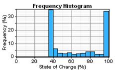
Battery
|
Quantity |
Value |
|
String size |
1 |
|
Strings in parallel |
16 |
|
Batteries |
16 |
|
Bus voltage (V) |
4 |
|
Quantity |
Value |
Units |
|
Nominal capacity |
122 |
kWh |
|
Usable nominal capacity |
73.0 |
kWh |
|
Autonomy |
135 |
hr |
|
Lifetime throughput |
169,098 |
kWh |
|
Battery wear cost |
0.502 |
$/kWh |
|
Average energy cost |
0.000 |
$/kWh |
|
Quantity |
Value |
Units |
|
Energy in |
2,176 |
kWh/yr |
|
Energy out |
1,806 |
kWh/yr |
|
Storage depletion |
73.0 |
kWh/yr |
|
Losses |
297 |
kWh/yr |
|
Annual throughput |
2,019 |
kWh/yr |
|
Expected life |
12.0 |
yr |

Inverter
|
Quantity |
Inverter |
Rectifier |
Units |
|
Capacity |
3.00 |
3.00 |
kW |
|
Mean output |
0.49 |
0.00 |
kW |
|
Minimum output |
0.00 |
0.00 |
kW |
|
Maximum output |
2.60 |
0.00 |
kW |
|
Capacity factor |
16.3 |
0.0 |
% |
Grid Extension
|
Breakeven grid extension distance: |
9.04 |
km |
Appendix 5: Prices
|
Solar panels |
|||||
|
Name |
Panels |
Effect
- kW |
Price
inc installation cost |
Replacement |
www |
|
Sanyo
HIP-230HDE1 |
1 |
0,218 |
kr 7.703 |
kr
8.703 |
|
|
Sanyo
HIP-230HDE2 |
5 |
1,09 |
kr 36.000 |
kr
41.000 |
|
|
Sanyo
HIP-230HDE3 |
10 |
2 |
kr 66.375 |
kr
76.375 |
|
|
Sanyo
HIP-230HDE4 |
20 |
4,36 |
kr 124.800 |
kr
144.800 |
|
|
Battery for battery bank |
|||||
|
Name |
Quantity |
Price |
www |
|
|
|
Surrette
4KS25P |
1 |
4.745 |
|
|
|
|
Surrette
4KS25P |
5 |
21.353 |
|
|
|
|
Inverter |
|||||
|
Name |
kW |
Price |
www |
|
|
|
Fronius
IG 30 Inverter |
3 |
9420 |
|
|
|
|
Fronius
IG 40 Inverter |
4 |
15233 |
|
|
|
|
Windturbines |
|||||
|
Name |
Rate
output |
Total
height |
Price |
www |
|
|
BWC
XL.1 |
1000
W DC |
9
m |
kr 13.800 |
|
|
|
SW
Whisper 500 |
3000
W DC |
16
m |
kr 42.500 |
|
|